PixelLM:Pixel Reasoning with Large Multimodal Model

Abstract

While large multimodal models (LMMs) have achieved remarkable progress, generating pixel-level masks for image reasoning tasks involving multiple open-world targets remains a challenge. To bridge this gap, we introduce PixelLM, an effective and efficient LMM for pixel-level reasoning and understanding. Central to PixelLM are a novel, lightweight pixel decoder and a comprehensive segmentation codebook. The decoder efficiently produces masks from the hidden embeddings of the codebook tokens, which encode detailed target-relevant information. With this design, PixelLM harmonizes with the structure of popular LMMs and avoids the need for additional costly segmentation models. Furthermore, we propose a token fusion method to enhance the model's ability to differentiate between multiple targets, leading to substantially improved mask quality. To advance research in this area, we construct MUSE, a high-quality multi-target reasoning segmentation benchmark. PixelLM excels across various pixel-level image reasoning and understanding tasks, outperforming well-established methods in multiple benchmarks, including MUSE, and multi-referring segmentation. Comprehensive ablations confirm the efficacy of each proposed component. All code, models, and datasets will be publicly available.

Model Architecture

PixelLM features a streamlined architecture, comprising four main parts: i) a pretrained CLIP-ViT vision encoder \( \mathcal{I} \) which aligns with text, ii) a large language model \( \mathcal{F} \), iii) a lightweight pixel decoder \( \mathcal{D} \) and iv) a segmentation codebook \( C_{\text{seg}} \). PixelLM processes image \( x_{\text{img}} \) and query text \( x_{\text{txt}} \), yielding interleaved text description and corresponding masks for varied target. At the core of PixelLM is the novel lightweight decoder and the holistic segmentation codebook. The codebook contains learnable tokens which encode contexts and knowledge pertinent to targets referencing at different visual scales. The pixel decoder then produces target masks based on the hidden embeddings from the codebook tokens in conjunction with image features. Thanks to this design, PixelLM can generate high-quality masks without external segmentation models, significantly boosting its efficiency. Furthermore, we propose a target refinement loss to enhance the model's capability of differentiating between multiple targets, thus further improving the mask quality.

Overview of the proposed PixelLM model architecture. (Left) Overall architecture. (Right) The proposed lightweigh pixel decoder. Trainable LoRA parameters are incorporated into the LLM. All parameters except those for the CLIP encoder and LLM are trainable.

Segmentation codebook

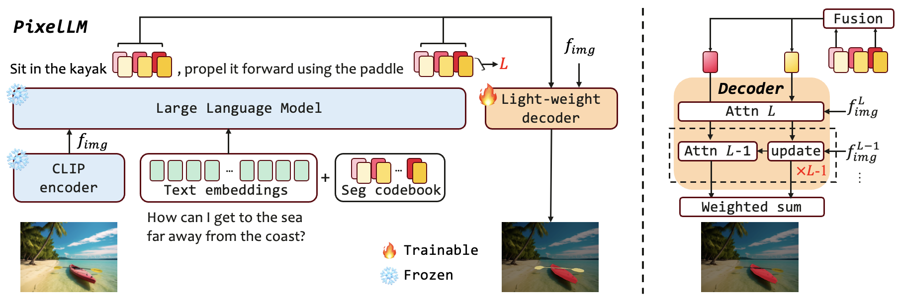
Specifically, the codebook consists of multiple token groups, each corresponding to a semantic scale of visual features from the image encoder. Formally, we define \(C_{\text{seg}} = \left\{ c_n^{\ell} \in \mathbb{R}^d \right\}_{n=1,\ell=1}^{N,L}\), where \(L\) and \(N\) denote the number of visual scales and tokens per group, respectively, and \(d\) represents the hidden dimension in LMMs. For clarity, we first set \(N=1\) and expound on how the codebook tokens are integrated within the LMMs to encode requisite information for target mask generation.

For an input image \(x_{\text{img}}\), the vision encoder \(\mathcal{I}\) extracts a spectrum of multi-scale visual features \(I_{\text{img}} = \{ I_{\text{img}}^{\ell} \}_{\ell=1}^{L}\) from \(\mathcal{I}(x_{\text{img}})\), comprising \(L\) visual features output at select layers of \(\mathcal{I}\). The output of the final layer, \(I_{\text{img}}^{L}\), encapsulates global image information and is transformed into the language space via a vision-to-language projection layer \(p_{V\rightarrow T}\). Simultaneously, a vision-to-decoder projection \(p_{V\rightarrow D}\) transforms all \(I_{\text{img}}\) features, resulting in \(f_{\text{img}} = \left\{f_{\text{img}}^{\ell}=p_{V\rightarrow D}(I_{\text{img}}^{\ell})\right\}_{\ell=1}^{L}\). The codebook tokens, combined with the input image and text, are then processed by the LLM to generate interleaved response \(y_{\text{res}}\) in an auto-regressive way: \begin{equation*} y_{\text{res}}=\mathcal{F}(p_{V\rightarrow T}(I_{\text{img}}^{L}),x_{\text{txt}}, C_{\text{seg}}). \end{equation*} To help understand this process, consider an example of text query ''Segment the apple on the left''. Then, the output \(y_{\text{res}}\) contains \(L\) tokens of \(C_{\text{seg}}\): '' The apple is \(c^1,\dots,c^L\)''. The corresponding hidden embeddings (i.e. the output of last layer of \(\mathcal{F}\)) of \(C_{\text{seg}}\) are represented as \(h=\left\{h^{\ell}\right\}_{\ell=1}^{L}\), which are inputs to the pixel decoder \(\mathcal{D}\) alongside image features \(f_{\text{img}}\) for mask generation. Each token interacts with the image feature at its corresponding scale.

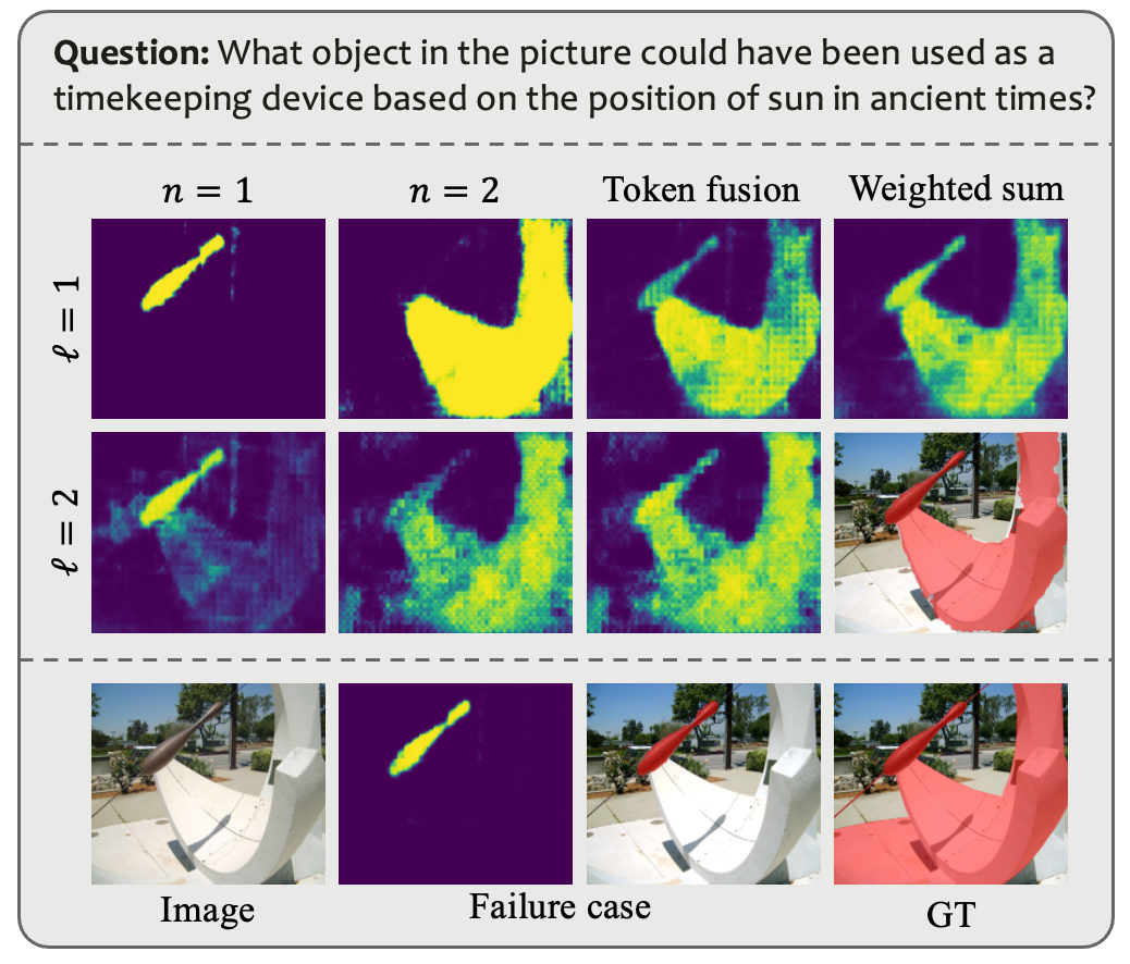
We then set \(N>1\) and explain the rationale. As shown in the upper right figure, scenarios featuring multiple targets or inherent complexity challenge the capacity of a single token to fully encapsulate target semantics, even though the LLM can provide accurate textual responses. In the figure, the segmentation codebook example comprises two scales with two tokens each. Each attention map results from the interaction between one token and its corresponding image feature in the decoder. The first two rows depict the token fusion mechanism, while the final row demonstrates a failure case arising from the utilization of only one token.

To enhance the model's interpretative ability in complex reasoning scenarios, we propose a token fusion mechanism that utilizes multiple tokens within each scale group, i.e. \(c^{\ell} = \left\{c_n^{\ell}\right\}_{n=1}^N\). Prior to decoder, a linear projection layer \(\phi\) is employed to transform the hidden states of grouped tokens into \(h^{\ell}=\phi(h_1^{\ell},\dots,h_N^{\ell})\). The figure illustrates the utilization of multiple tokens per group. The visualization of each attention map post decoder reveals that disparate tokens yield complementary information, culminating in enhanced mask compared to a single token setting.

Pixel decoder

We design a novel and lightweight pixel decoder \(\mathcal{D}\) that are engineered to adeptly harness the multi-scale features from the vision encoder. This decoder is tasked with learning the transformation of these features, in conjunction with the hidden embeddings from \(C_{\text{seg}}\), into precise segmentation masks. Such an design obviates the need for extra costly segmentation models like SAM, thus significantly improving efficiency.

As depicted in the right panel of the model architecture figure, \(\mathcal{D}\) consists of \(L\) attention blocks \(\left\{Attn^{\ell}\right\}_{\ell=1}^{L}\), each corresponding to distinct scales of image features and the codebook. For each targeted mask generation, \(\mathcal{D}\) sequentially produces a mask score map \(m^{\ell}\) at each scale \(\ell\), which then directs the model’s attention to regions of higher relevance in the subsequent scale \(\ell - 1\). This strategy works by guiding the model to focus on areas with high confidence scores in \(m^{\ell}\), thereby facilitating more accurate mask generation. \[ \begin{equation*} \begin{aligned} f_{img}^{\ell^{\prime}} &= \left\{ \begin{array}{lc} f_{img}^L&\ell=L \\ f_{img}^{\ell} \odot (\sigma(m^{\ell+1}) + 1) &\ell< L \end{array} \right. \\ m^{\ell}&=Attn^{\ell}(h^{\ell},f_{img}^{\ell^{\prime}}). \end{aligned} \end{equation*} \]

We then set \(N>1\) and explain the rationale. As shown in the upper right figure, scenarios featuring multiple targets or inherent complexity challenge the capacity of a single token to fully encapsulate target semantics, even though the LLM can provide accurate textual responses. In the figure, the segmentation codebook example comprises two scales with two tokens each. Each attention map results from the interaction between one token and its corresponding image feature in the decoder. The first two rows depict the token fusion mechanism, while the final row demonstrates a failure case arising from the utilization of only one token.

where \(f_{img}^{\ell^{\prime}}\) is the modulated feature at scale \(\ell\), \(\sigma\) is sigmoid function and \(\odot\) is element-wise multiplication. Finally, we learn the weighting factors \(\gamma=[\gamma^{\ell}]_{\ell=1}^{L}\) to combine mask maps at all scales to get the final segmentation result: \(\hat{M}=\sum_{\ell=1}^{L} \gamma^{\ell}m^{\ell}\) where \(| \mathbf{\gamma} | = 1\).

Multi-reasoning segmentation dataset (MUSE)

To facilitate model training and evaluation in this area of research, we develop MUSE, the first comprehensive multi-target reasoning segmentation dataset. MUSE stands out with its open-set concepts, detailed object descriptions, complex multi-target question-answer pairs, and instance-level mask annotations. Specifically, we feed all the instance category names and corresponding bounding box coordinates in the image to GPT-4V. Using carefully crafted prompts, GPT-4V autonomously selects instances to construct question-answer pairs relevant to the image content.

The left panel illustrates the prompt employed in our GPT-4V data generation pipeline. The right panel showcases an example of the generated data.

Dataset statistics

A total of 910k high-quality instance segmentation masks are selected from the LVIS dataset, along with detailed textual descriptions based on image content. Utilizing these instances, we construct 246k question-answer pairs, averaging 3.7 targets per answer. This dataset is then divided into three splits: train, val, and test, containing 239k, 2.8k, and 4.3k question-answer pairs, respectively. The test split comprises two parts: the number of targets involved in the question are less or more than three.

Category statistics. There are over 1000 categories in MUSE from the original LVIS dataset, and 0.9 million instances with unique description that vary based on the context of the question-answer pairs. Figure (a) shows the number of instances per category on all question-answer pairs. The distribution inherit the low-shot nature of LVIS.

Token count. Figure (b) presents the distribution of instances by token count in their descriptions, highlighting a wide range that exceeds 100 tokens in the most extensive cases. These descriptions are not limited to simple category names; rather, they are substantially enriched with detailed information about each instance, encompassing aspects like appearance, attributes, and relationships with other objects, thanks to our GPT-4V-based data generation pipeline. The depth and variety of information in the dataset bolster the trained model's generalization capabilities, enabling it to effectively address open-set questions.

Target count. Figure (c) presents statistics on the number of targets in each question-answer pair. The average number of targets is 3.7, with the maximum number of targets in a single pair reaching up to 34. This number can cover most scenarios of target reasoning for a single image.

Evaluation

Let us denote by \(M=\{M_g\}_{g=1}^G\) the ground truth set of \(G\) objects, and \(\hat{M}=\{\hat{M_k}\}_{k=1}^K\) the set of \(K\) predictions. Motivated by ~\cite{detr}, assuming \(K\) is not equal to \(G\), we use \(\varnothing\) (no objects) to pad the smaller set and both sets finally have size \(P={\rm max}(G, K)\).

(1) We find a bipartite matching between these two sets by searching for a permutation of \(P\) elements, \(\sigma\in\mathfrak{S}_P\), with the lowest cost: \begin{equation*} \hat{\sigma} = \mathop{\arg\min}\limits_{\sigma\in\mathfrak{S}_P} \sum_{i}^{P} \mathcal{L}_{match}(M_i, \hat{M}_{\sigma(i)}) \end{equation*}

where \(\mathcal{L}_{match}(M_i, \hat{M}{\sigma(i)})\) is a pairwise matching cost between ground truth \(M_i\) and a prediction with index \(\sigma(i)\). We compute this optimal assignment efficiently with the Hungarian algorithm. We define \(\mathcal{L}_{match}(M_i, \hat{M}{\sigma(i)})\) as \(\mathcal{L}_{bce}(M_i, \hat{M}{\sigma(i)}) + \mathcal{L}_{dice}(M_i, \hat{M}{\sigma(i)})\).

(2) Based on the matching results, we modify the generated response \(y_{res}\) to \(y_{res}^{\prime}\): since each \(\hat{M}_i\) originates from a segmentation token sequence in \(y_{res}\), we replace each sequence with the GPT-generated description of \(M_i\).

(3) We use a carefully designed prompt for GPT-3.5 to assign a score \(s_i\) to each \(\hat{M}_i\) in the answer in a single step. An example of this methodology is depicted in the above figure. The empty predictions are directly scored with 0.

The above three steps assess the model's capability to generate outputs where masks are intertwined with text descriptions, and evaluate how accurately these masks correspond to their respective text descriptions. Then we evaluate the quality of the masks.

(4) The final IoU of each prediction is: \begin{equation*} \begin{aligned} {\rm Intersection}_i &= \left\{ \begin{array}{lc} {\rm Intersection}_i &s_i>0.5 \\ 0 &s_i\leq0.5 \end{array} \right. \\ {\rm IoU}_i &= {\rm Intersection}_i / {\rm Union}_i \end{aligned} \end{equation*} And the final IoU\(_{img}\) of each image is: \begin{equation*} {\rm IoU}_{img} = \sum\nolimits_i {\rm IoU}_i / P \end{equation*} Based on the IoU scores, we can calculate gIoU and cIoU metric like referring segmentation dataset.

BibTeX

@misc{ren2023pixellm,
  author= {Zhongwei Ren and Zhicheng Huang and Yunchao Wei and Yao Zhao and Dongmei Fu and Jiashi Feng and Xiaojie Jin},
  title = {PixelLM: Pixel Reasoning with Large Multimodal Model},
  year={2023},
  eprint={2312.02228},
  archivePrefix={arXiv}
}